These components are required:
Resistance 3.3 kΩ | 4.7 kΩ | 4x 22 kΩ from the AZ resistor kit
Electrolytic capacitor 10 µF from the AZ Electrolytic Capacitor Set
Potiometer 10 kΩ | 10 gang poti
2 LM 358 operational amplifiers
Electronics retail trade
Multiple measuring device with measuring areas up to 100 MA and 50/100 µA
Measuring structure for characteristic determination
In the first post on the topic „Determine transistor characteristics with the TDMM“We got to know the basics as well as a PWM ramp generator and the difference amplifier.
We use the circuit for our experiments (Figure 1), whereby we take off the tensions and/ or currents in different places depending on the experiment.
Our examinee, the transistor BC548C (also every other NPN transistor) accompanies us through this post. If you want to experiment one more, you can expand the project to JFET and MOSFET transistors or other semiconductors and can therefore do a lot of interesting attempts.
Measurement structure ube - Route
If I can assume that the rectifier diode is known as a component, then you can see such a diode between the base and emitter of a transistor in the transistor. In fact, the cover of a transistor has diode properties. It only leads the current in one direction. At the NPN transistor, he flows from the base to the emitter. From a certain voltage, for transistors (and diodes) based on silicon, it is around 0.7 V, the diode begins to guide. Only then can electricity flow.
Let's take a look at the simple measurement structure for which we use the transistor, the PWM ramp generator, the differential amplifier and the TDMM:

Image 1: Measurement structure UBE - route
The PWM ramp generator provides a voltage via the 100 kΩ resistance R6 to the base of the transistor. We measure the base current using the difference amplifier and observe it depending on the voltage andbe Between the base and emitter. The transistor does not require a collector resistance and no power supply. He works as a diode.
Practical implementation
In theory, this measurement is very easy. We determine the base current from the voltage difference above the resistance R6. IB = UR6/100,000 [a] (Ohmsche's law: i = u/r).
The base current is very small. It controls the much larger collector current, as we have already seen in Part 1. It is best to count on Ampere in millionths: 1µA = 0.000001 A.
We record two tensions for the measurement: the Ube between the base and emitter (= GND) and the voltage UR6 above resistance R6 (which is proportional to the base current). UR6 Measures our difference amplifier.
We have already done half of this task. In contribution section 1 we carried out a linerarity check (Figure 5) for the PWM ramping generator and can indicate which pulse width ratio C (0… 255) which output voltage is generated, our Ube. However, I recommend checking the calibration and creating a table for 4… 5 PWM values.
We then only need to measure the base current for every value to which we set the PWM ramp generator.
Measurement of the diode with PWM ramp generator and oscilloscope
Although not every electronics technician has an oscilloscope, I would like to briefly introduce this elegant and simple method. In this case you let the ramping generator run freely and connect the oscilloscope instead of the TDMM to the outcome of the difference amplifier. Now you can see the dio thinking line immediately:

Picture 2: UBE stretche oscillogram
There is a sketch called "Rampenerator_10er_ steps", which starts the ramping generator at 0 and runs up to 250. On the oscillogram you can see quite well how the diode effect lets the base current curve rise steeply.
There is a potentiometer on the PWM ramp generator to set the reinforcement. This allows you to choose the trigger point at the oscilloscope exactly. One more tip: The 10 µF capacitor is periodically through the instructions
analogWrite(pin, 0); // Spannung = 0, Kondensator entladen
delay(50); // Zeit für Kondensatorentladung
unload. Depending on the election of the ELKO, this is not always enough to get under the 0.7 V threshold of the cover. That is why - only for this one measurement - I switched a 4.7 kΩ resistance to the capacitor in parallel in order to unload it faster. With that, recharging is slower. The oscillogram shown above could be created with this compromise.
You can see on the oscillogram that the lowest voltage is not exactly 0 volts, but about 0.2 V. The vertical axis of the oscilloscope is set to 0.5 V per skal section. At approx. 0.7 V - almost exactly on the horizontal, dashed orange line - bends the line upwards and becomes steeper. This is how the diode status of the corner of our transistor is presented.
Automated measurements with a python script
Now we want to control the PWM ramp generator with a Python script on our computer and measure it at the same time with the TDMM. In part 1 we had already met the three new instructions for the TDMM. We had provided the associated .ino file.
Now we rebuild the PWM ramping generator so that it can be controlled by a simple instruction via the USB-Serial interface. Again we use the Command processor that you know from my projects. You can find the code for this in the file “triggerable_rampenerator.ino ". At the start, the module in addition to the help command still offers the simple instruction" Up XXX ". "Up" is the command, followed by an empty space and an integrated 0… 255. This value determines the voltage at the output of the PWM ramp generator. "0" means: "No tension". "255" means "maximum voltage".
Since we have installed a potentiometer in our module, we can enter an instruction "Up 255" in the IDE and then set the value we want to use for measurement with the potentiometer. We need this function the same.
The python script
The measurements are carried out with a Python script that takes on the following tasks:
- Connection to the two serial interfaces
- Control of the devices
- Send instructions to both devices
- Read, save and process data of the TDMM data
I used the Thonny-IDE with Python 3.11.1 for the measurements. Python is open source and freeware. It is available on Win, Linux and MacOS. When download, please take a close look that a "clean" website is used for download, e.g. www.python.org
Let's take a closer look at this script:
In the first three lines the libraries are "Serial" for USB communication, "Time" for time and queue as well as "CSV" for CSV data preparation.
After that, two ports are defined that contain the respective addresses of the serial interfaces of their devices. To find these interfaces, you can use two quite simple Python commands from the Command line >>> From work, such as such:
>>> import glob
>>> glob.glob('/dev/tty.*')
['/dev/tty.Bluetooth-Incoming-Port', ‚/dev/tty.usbserial-110']
In the command line, import the "Glob" library. If necessary, this library must first be installed via the library manager.
In the second command line, ask Glob about all devices with "Tty" properties. Please pay attention to the exact spelling. You will receive a list of serial devices. The first device is the Bluetooth interface that you also know from the Arduino IDE. In this case, the second device is the port of my TDMM. After that, I connect the PWM ramping generator and I will renew globs query. Then get the address "/dev/tty.usbserial-30“, My ramp generator.
The ports of your devices will probably look different. Please enter in line 6 and 7.
My ports are connected to a MacBook Air. At Win they look different, very similar to Linux, as presented here.
A global array MW () for the measured values is also created.
We have the main program Main () below that accepts your instructions. In front of it are the different functions:
Open_Serial (port): Opens the communication sport and reports if necessary. Mistake
write_data (ser, data): Sends data to a port "ser"
Clear_MW (): Deletes the content of the measurement value ray
print_mw (): Issues the content of the measuring value ray on the screen
Measure (Ser1, Ser2): If the measurements carries out, controls the devices, the data stores
csv_maker(): Exports the measurement data as CSV In the file under "CSV_File_Path"
Main(): The main program with command selection.
Some readers are certainly "at home" in Python. For them, the script will certainly be readable and understandable immediately. Otherwise, I suggest it simply to use it like a measuring device that you don't necessarily need to know what it looks like inside.
The script connects to the two devices after the start and presents a functional menu:
(l) read, (s) write, (c) mw lÖ(D) Meat (M) Measure, (V) CSV file (Q) Quit "
The instruction S expected data for both devices. L Only read data from the TDMM
You can with S Send the instruction "SO" (Serial Output Off) to the TDMM and at the same time "Up 0" (no output) to the PWM ramp generator. Then you give once L one and gets the message from the TDMM that the serial output was switched off. Without this small procedure, you will otherwise get an error message when starting a measurement, because the serial buffer also contains the textant word of the TDMM on the "SO" instructions.
Should be with the start of the exhibition program M but still An error message appear (because the script expects a number but receives a text report), you just restart.
The program should always be ended with "Q" for "Quit" so that the script can close the ports clean. Otherwise there can be difficulties in a renewed connection.
1. Attempt: automated measurement of the diode route
Now that we have provided the tools, we carry out the first measurement. We repeat the measurement that we have carried out with the oscilloscope. To do this, we carry out the measurement with a small variation.
When we first tried our first attempt, we did not switch the transistor collector, but only used it as a diode. Now we take a closer look. The transistor is used for our measurements in the so -called emitter circuit. The emitter is at the most negative level of voltage, with us to zero volt (mass, also called GND).
The collector is connected to the plus pole of the power supply via a work resistance, in our example with +5 V and a resistance of 680 Ω. This situation reflects Figure 4:

Fig. 4:
The characteristic of the date is by no means independent of the operating tension UCC of the transistor. She changes with UCC! In this example we decided to measure with UCC = 5V.
Calibration of the PWM ramp generator
We invite the sketch "triggerable rampenerator" and use the "Up 255" instruction to set the highest possible tension, which we control with the TDMM.
The value of the ramping generator is now set to 5.0 V. The measurement clamp of the TDMM is now connected to the output of the difference amplifier and the script started.
Measurement of the date
The script connects to the two devices. When an error message comes, simply click on "Stop" in Thonny IDE and start again. Then the measurement that runs through in 25 steps begins.
At the very end you can use the results with the instruction D Watch and then the data with the instruction V export as a CSV file. The file name is defined in line 70 of the Python script.
You open the CSV file in a spread of the spreadsheet program. Most of the time it is still a click of the mouse to the finished diagram that - not astonishing - looks confusingly similar to the oscillogram:

Image 5: Measuring result
We find that the "breakthrough voltage" is again around 0.7 V.
2nd attempt: measurement of the power reinforcement β or hFe
Both names stand for the power reinforcement of the transistor. β = IC / IB . A control current IB In the event of a predefined voltage andCE A collector current IC. This is one of the most important parameters of the transistor because it tells us how well it can be used as an amplifier. With our BC548C, β is 500 - 900.
The power reinforcement depends on some other factors, e.g. on the ambient temperature, the frequency of the signal to be reinforced and - as mentioned - on the operating voltage or UCE .
The measurement structure remains unchanged, only that this time we the base current IB and the collector current IC determine. Since we already know which base current flows at which PWM value, this preparatory work makes the measurement easy. We choose 12 V as the operating voltage, because in part 1 of the contribution we determine the linearity of the PWM ramp generator with this voltage and the values for Ube and iB have determined. If necessary, simply let the python sketch go through it again and secure the results for this measurement.

Image 6: IC AbhäNgig from IB
We only need the tension andCE To measure for each PWM value e.g. of 0… 250. From uCE The voltage is calculated above the resistance R8. The collector current is then iC = (12V - uCE)/R8.

Figure 7: Beta at UC_12V
In my measurement, the supply voltage was 12.2 V. The values are calculated accordingly. You can see that the transistor offers a large area in which the power reinforcement forms one straight, so it remains largely the same. It is said: "The characteristic line is linear in this area".
With very small base currents, the reinforcement is low. Then the large, linear area follows, the actual work area of the transistor as an amplifier. If the base current increases even further, the reinforcement becomes lower again, the characteristic line flatter. The transistor "goes into satiety". It becomes an electronic switch, a task for which transistors are often used.
3. Experimental: Determination of the starting characteristic crowd
The determination of the initial characteristic crowd needs a little more preparation and is more demanding than the first two attempts.
The transistor is connected to an emitter and collector to a voltage source that a variable collector emitter voltage UCE specifies. With a fixed base current IB becomes uCE From 0 volts to 10 volts gradually increased. This time we use 10 V to be able to calculate more easily. The basic current causes an I toC, which as a function ("depending") of UCE is observed.
We observe iC With three different base flows and thus learn the area of application of the transistor quite well, e.g. as a component of an amplifier.
The associated circuit looks like this:

Figure 8: Measuring structure Starting characteristic
Under the point "These components are required", we have proposed a 10kΩ potentiometer that can be set from 0 to 10kΩ with 10 revolutions. With this application, it does particularly well and is expressly recommended.
The potentiometer divides the input voltage, which is led to the base of the transistor from the potentiometer with a measuring range of 50 µA and 100µA and the 10K resistance R9. If a micro -meter with a somewhat "coarser" measuring range, maybe only 250 µa, the measurement is generally the same. The fault bars are then a little longer.
The transistor continues to work in emitter circuit. He has now received a 10Ω resistor R10 between emitter and mass (GND). We expect a collector current of a maximum of 100 mA. The BC548C is no longer tolerated. We calculate: u = i*r = >> U = 0.1a * 10 Ω and get with the highest possible Collector current on R10 a voltage of 1 V. In this way we want to use the TDMM the IC measure. In fact, we will burden the transistor with less than 30 mA.
To make sure that our TDMM measures between 0… 1 V with sufficient linearity and accuracy, I made an attempt and switched a 6 ½-digit digital voltmeter (HP34401A) in parallel. The measurement error of the TDMM also remains with a voltage of 0.1 V below 5%. This is absolutely sufficient for our purposes.
Precial attempts for better understanding
Blocking behavior of the CE route
If you make such an attempt, you want to learn more than the standard textbook shows. We want to know: How well does the transistor block when we lay the base of the transistor to mass (GND)? Which residual current flows?
If you try it out, please turn the UCE At your power supply to up to 30 V, while measuring the electricity from the power supply to the transistor at the same time as the millia emperor. In fact, you will find that no measurable electricity flows.
Behavior of the CE route in the passage area
If you convert the circuit according to Figure 8, connect the 10K potentiometer and connect it to the base of the transistor via the pre-resistance R9. Be sure to set the potentae to zero. Measure whether the voltage behind the potentiometer is really zero before connecting the transistor collector to the power supply!
Make the following clear: The transistor hangs on your power supply, which is set on 12 V. The electricity through the CE route is limited only by the 10Ω resistance. At 12 V and 10 Ω the possible electricity is limited to 1.2 a - i.e. 1,200 mA by the transistor. The data sheet of the BC548C tells us that a maximum of 0.1 a - 100 mA - are permitted. So there is a chance to create a foul -smelling cloud of smoke and destroy the transistor. So watch out!
We have a transistor with a β of at least 500. It can't be more!
They now switch a millia mapers, measurement range 100 mA in the collector circle between power supply and the collector.
If you are sure that everything is right, turn on the measurement structure now and observe the milliapers in the collector circle. If you now carefully open the 10-speed potentiometer from the zero position, you will quickly see the collector current. It gives them a feeling of how sensitive the transistor is and how enormously its reinforcement. If you measure the base current at the same time, you canB/IC Understand the measurement again.
We prepare the characteristic measurement
An old electronics wisdom says: "Anyone who measures measures crap". So that we are not doing this, we reinsure that the measurement structure and the participants do devices what we want.
Calibrate the PWM ramp generator again
We close the trigger ramping generator as a voltage source for UCE to the transistor collector, as shown in Figure 8. The trigger ramping generator should uCE deliver and it will be the collector current IC flow that the operating amplifier has to apply in our ramp generator.
To do this, we look into the data sheet of the LM358 - operational amplifier and find that this can be a maximum of 40mA. The tension is not a problem. But the output current is limited.
It is recommended not to use the maximum values - we see why.
We start our ramp generator and give the instructions Up 250 a. I recommend a supply voltage around 12 volts, the value is uncritical. Now we set the output voltage of the ramping generator to almost exactly 10 volts. The potentiometer for the basic preload is completely zero. No basic current should flow and therefore not Ic. The ramp generator is not burdened.
|
IC |
IB |
UCE |
|
0 MA |
0 µa |
10.00 V |
|
10 mA |
20 µa |
9.91 V |
|
20 mA |
43 µA |
9.77 V |
|
30 mA |
67 µa |
9.62 V |
Now it will be interesting. Gradually we - carefully - increase the basic preload and write down the results for the actual UCE (Measure with the TDMM). Here is my result:
We recognize that the ramping generator is not a perfect source of tension, but has a so -called "internal resistance". This is quite normal and doesn't bother us. But we now know that with increasing electricity there is no 10 V more on the collector, but only 9.62 BO. An error of less than 5%. But: errors add up in many cases.
Our ramp generator has grown the task and can be used sensibly under the boundary conditions described.
Because the operating amplifier limits the possible collector current to 40 mA, the transistor lives safely. It cannot be destroyed by the measurement arrangement.
The operating amplifier LM358 itself is permanently short and against overload.
Measurement of the UCE - IC - characteristic
Since weCE - IC - Want to watch the course of various settings of the base current, a characteristic line arises for every fixed base current. Together they are called a “characteristic group”.
The actual measurement can take place as follows:
1. Please call the TDMM_Messprogramm_v4.py. I chose the settings there so that the program performs 10 measurements, starting at UCE = 0 V to UCE = 10 V. Feel free to choose other settings.
2. Choose a base current that lies ≤ 60 µa. My choice is 20 µa, 40 µa, most recently 60 µa.
3. Now start the measurement program and first enter the instruction "L" for "Reading.
4. With "M" you start the automated measurement.
5. Now take a look with "D" (display) whether the measured values have been transferred to the results array and whether the values seem sensible to them. If this is the case, please transfer the results into a CSV file with "V". You define the name of this file in line 70 of the Python script.
6. Now delete the result array with "C" and set a different base current. Restart the measurement with "M". Everything starts from the front.
7. To finish all measurements, please use the "Q" (Q) instruction, also to close the serial ports again.
The reward for the effort is a characteristic of a characteristic, which you will easily create with that of your spreadsheet calculation. Please note: Some spreadsheets need the comma as a decimal separator, the English/American. Solutions use a decimal point. Possibly. Search and replace globally.

Figure 9: Starting characteristics group
Conclusion and outlook
What you got to know in these two blog posts is part of the basic knowledge of electronics and is important to understand. The transistor is the basic element of all electronics. It is often carried out as a MOSFET today and is probably millions of times and extremely compact in her pocket. Knowing the basics is always good and is fun.
Have fun and success when implementing the project and
Until the next blog post
Her Michael Klein